Data Presentation: Value-Added GeoPDFs

When I initially heard about GeoPDF I thought it sounded like a good enabling technology for people without advanced geospatial expertise or access to the appropriate software. After all, anyone can view a PDF. Typically I thought of it in the context of viewing RGB orthophotos... Fast-forward to the present: lately I've been thinking about ways of presenting fused data, and this is where GeoPDFs came to mind. In particular I wanted to present terrain and image data.

For input data I started with some edge-matched orthophotos of Sligo, Ireland and processed XYZ LIDAR data of the same area (data courtesy of OSi). I processed the data in LPS and IMAGINE, which basically involved importing the LIDAR data and converting it to the IMAGINE IMG format, and then creating a shaded relief map out of it. For the imagery I mosaiced several tiled input images into a single orthomosaic. The processing resulted in three products: an RGB image file, a shaded relief image, and a DEM. To put them all together I used the "Layer Stack" function in IMAGINE, which resulted in a 7-layer 8bit IMG file.


Next, I converted the IMG to a GeoPDF. This was a painless process and produced a 7-layer PDF file. My input file covers a fairly broad area and was a few gigs (2.7GB to be precise) in size so I used a JPEG compression quality factor of 60, which for visual analysis creates a fairly sharp-looking image in a PDF format with a much-reduced size of 122MB. This allowed me to open up the image in Adobe Reader and view the image.

Because the first three layers of my image are the RGB orthomosaic, this is what is displayed when opening the PDF in Adobe Reader. I also have the GeoPDF Toolbar (recently renamed to TerraGo Desktop) loaded as well for various measurement and manipulation functions:

(click any of the screen captures for larger views)

By clicking on the "Layers" button I could adjust the band combinations for RGB to display the shaded relief.


It was also possible to display various fused results. In this example I am displaying Red and Green from the orthomosaic and then loading the DEM into the Blue channel. This means the colors are skewed but the benefit is that you can see the image feature details and also get a notion of the high-relief areas. In this case high relief shows up as dark blue, and the absence of blue indicates low-relief (e.g. the upper left areas).


Note that many kinds of band combinations/visualizations are possible with this fused product.

Many thanks to Adam Estrada for assisting with the GeoPDF part of this workflow. I also plan on making the dataset available soon (I'll hopefully get it uploaded tonight).

National Agriculture Imagery Program (NAIP) Best Practice Report

A couple of days ago I stumbled across a report put together by ITT for the USDA's APFO group outlining suggestions for improving NAIP image quality. If you're interested in the radiometric processing of aerial photography, this is a must-read. The document outlines image collection guidelines (e.g. optimal flying conditions), the assessment of imagery quality, and image processing recommendations. Some of the material (e.g. orthorectification) is relatively high-level, but the sections on radiometry are great. Also be sure to check out the end of the document, which features a set of screen captures depicting radiometric problems and solutions (pre and post-processing) for image noise, sharpness, clipping, contrast, saturation, and color channel registration.

One thing to note is that NAIP imagery is generally available to the public. Aside from the USDA/NRCS Geospatial Data Gateway, it is also accessible from a number of regional/state-level organizations. A great resource for free orthophotos, NAIP and otherwise, is the World Wind Central section on the topic.

For some practical advice see Jarlath O'Neil-Dunne's recent post (and particularly the video) on the methodology and benefits of using the Vermont 2008 NAIP imagery in a GIS.

Dodging: An Art and Science

A couple of weeks ago I wrote a post covering an introduction to dodging. It outlines typical radiometric problems, introduced the concept of dodging, and then went into statistics generation.

Today I will focus on the actual dodging process. For the example data I will use some frame camera imagery covering Laguna Beach, California (from the LPS Example Data).

Here's a screen capture of the original undodged imagery:


It is apparent that the radiometry is uneven. In particular, the bottom right quarter of the image has a whitish hue. You can see that the hills should be the same color as the rest of the scene, but instead they are discolored and uneven throughout. In addition, there are several radiometrically inconsistent areas throughout the image. For example the urban area on the bottom-left looks completely washed out (lacking contrast), as is the area under development just above it.

After generating statistics (discussed in the previous post), the next step involves adjusting the correction parameters. After statistics describing the imagery have been generated, the dodging algorithm applies a "target" output value for each pixel. For example, the input DN value of one specific pixel band may be 125. After statistics are generated (describing the image or a group of images), the dodging process identifies a target "adjusted" pixel DN value. Then, constraints are used so that extreme changes to the imagery are not applied. Here are the ImageEqualizer constraints and correction parameters for the Laguna image above:

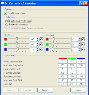
You can see that there are a few different categories. Here's how the options work:

• Band Independent: if checked, allows you to adjust bands independently. This is useful if your imagery is skewed in one band (e.g. your imagery has a "reddish" hue and you want to align the red band with the green and blue bands).
  
• The balancing options allow you to adjust the images individually or as a group. This is a useful option if you are adjusting images that have radiometric differences across the images. For example, if you have flight lines that were flown on different days with different lighting conditions you would definitely want to balance across images to even up the radiometry (if the final product is an orthomosaic).
• The brightness and contrasts sliders are relatively self-explanatory. You can adjust them for each band. The "undo" button will take you back to the default brightness/contrast value.
• The constraints section allows for control over how the dodging algorithm is applied to an image or group of images. It comes with pre-defined defaults (which you can see above). These parameters are critical for tweaking the image adjustments.

With the default dodging parameters applied, the input imagery above looks like this:
The original image is on the left and the dodged image is on the right. You can see that a lot of the problems in the original image have been resolved. However, by adjusting the parameters it can still be improved. The contrast is still fairly low, and the light area on the bottom right is still noticeable (although much less so).

In an attempt to improve it even more, I adjusted two of the constraint parameters. These were the "Maximum Contrast" and "Maximum Grey Shift" parameters - which are two highly critical constraints in any dodging process. The max contrast constraint has a default value of 1.3, which attempts to limit excessive contrast adjustment in low contrast areas. Increasing this value will bump up the limits on "target" contrast adjustments. Since the input imagery has some low-contrast areas, I bumped this constraint up to 1.8. Maximum Grey Shift applies a limit, by default 32, on how much a pixel's DN value can shift. For example, a specific pixel may have a DN value of 120 in one band. The dodging algorithm may determine that the "target" value should be 160 (e.g. it needs a pretty big adjustment). This constraint with the default 32 value will limit the final adjustment to 152. The reason for this is to limit extreme changes in the imagery. Since I could still see at least minor unevenness in the radiometry with the default constraints, I increased the max grey shift to 50.

Here is a screenshot previewing the original and dodged image (left) with my final dodging parameters (right).

In addition to changing the constraints outlined above, I also decreased the brightness a bit and bumped up the contrast (evenly across bands - I didn't adjust any single band more than another). This helped to reduce the washed out effect and produce an even scene.

Here's a close up of the urban area with a part of it under construction. You can see how the dodged image on the right has much better results. Grassy areas are green, roofs look correct, and the construction site doesn't look so washed out.


I used ImageEqualizer for dodging this example image, but the same dodging algorithm is also embedded as a color correction option in ERDAS MosaicPro. Applying dodging in MosaicPro will apply the results to the output Mosaic and will not impact the input images. This can be handy for "two-stage" dodging. For difficult radiometry, it is sometimes necessary to dodge the imagery twice: once right after scanning and once during (or after) the photogrammetric processing (e.g. during or after mosiacking).

Dodging: Intro and Statistics

One of the problems with creating seamless image mosaics or tiled orthophotos is "getting the radiometry right". What does that mean? Well, there are a lot of things that can turn a project sour when trying to make a good-looking final product. Some common radiometric issues are:

• Hotspots and vignetting: these are common in scanned aerial photography, where the sun's reflection causes a bright spots. Vignetting is where a darkening occurs towards the corners of the image. See here for a good vignetting description.
• Flightlines of imagery flown on different days or different times of the day. Some mosaicking jobs include images that were flown at either different times of the day, or on different days (with different weather conditions). This can be a difficult problem to deal with because the imagery of the adjoining flightlines may be completely different in terms of the sun angle, brightness level, cloud coverage, and so forth.
  
• Brightness problems. Another issue is when, usually due to on-board sensor settings, one color band's brightness level is either too high or too low. For example, the imagery looks "blue-ish" because the blue band brightness level is skewed. Panchromatic imagery may also be too dark or light and need adjustment. It is also possible for there to be brightness variation within on image.
  

See the image below for an example. Three of the corners are dark and the bottom of the scene is inconsistently light compared to the rest of the scene. Overall the radiometry is uneven.

For aerial photography, one tool that can be used to alleviate the above problems is a process known as dodging. While there may be other problems, such as atmospheric issues associated with satellite imagery, these may require the use of other tools.

So how can dodging help?

Dodging basically attempts to create a uniform spectral intensity within and across images. Dodging, in the traditional photography sense of the word, is about reducing the exposure in a portion of the image in order to make that portion appear lighter. In photogrammetric processing this completely digital process. There are numerous programs available to perform dodging, and they often share techniques.

From ERDAS we offer dodging capabilities in a few different applications, namely Leica MosaicPro and ImageEqualizer. Both of these applications use a dodging algorithm originally developed by LH Systems for use with the DSW scanner line (implemented in a program called Fastdodge).

In these applications, the processes for statistics generation are similar:

A set of statistics are calculated (e.g. mean, standard deviation), which are based on certain user-defined parameters. These include grid size, skip percentage, and the minification layer (aka pyramid layer) for the process to run on. Of these, both the grid size and minification layer can be quite critical for success.

1. Grid size defines the number of grid tiles in x and y for statistics to run on. For example, a grid size of 10 will result in 100 grid tiles (10 in x, 10 in y). Depending on the scene, this can have a big affect. For example, frames with relatively contiguous radiometry can use small grid sizes. "Complex" scenes, such as a frame containing water, urban, and rural/vegatated areas, usually require a higher grid size/density to prevent one radiometrically contiguous area from affecting another area. For example, consider a patch of dark green vegetation surrounded by say, lighter colored grain crops. If the grid size is significantly larger than the dark green patch, the output (depending on the constraints applied) will wash out the dark green because of the statistical influence of the DN values of the lighter colored grains. However, sometimes the problem outlined in this example can be impossible to avoid! This is why dodging is both an science and an art....
   
2. "Skip percentage" is generally referred to as an "edge trimmer" (e.g. the percentage of the image edge that will be ignored during stats generation). It is important not to confuse this with "skip factor", which generally refers to a certain factor of pixels to "skip" when calculating stats. Using a high skip factor can have the same effect as using a lower-resolution pyramid layer.

The "minification" (or pyramid layer) setting is used to define which minification layer (e.g. a reduced resolution version of the 1:1 image) to use for stats calculation. Using a lower-resolution minification layer will result in faster stats generation, but it needs to be used with caution because if you have a radiometrically-complex (e.g. lots of non-contiguous radiometry, or in other words a "busy" scene) using a low-res minification layer can skew the stats.